Lab Exercise 5: Solutions

TCP Congestion Control Revision (not marked)

Question 1. At 1 a loss was detected through triple duplicate ACKs, while at 2 a loss was detected through a timeout. Since a timeout is considered worse than triple duplicate ACKs, the congestion window is decreased more drastically (i.e. reset to 1).

Question 2. Region 3 coincides with slow start during which the congestion window increases exponentially.

Question 3. Region 4 coincides with Congestion Avoidance (or AIMD) during which the congestion window is increased conservatively as the connection slowly probes if there is further available bandwidth.

Question 4. During slow start, the window is increased more rapidly so that the connection can quickly discover the available bandwidth. This prevents wastage of resources.

Question 5. After the timeout experienced at 2, the congestion window is reduced to 1 and the threshold (ssthresh) is set to 1/2 the size of the window. The congestion window then quickly ramps up from 1 to the threshold (i.e. slow start). Following this the connection transitions to Congestion Avoidance (or AIMD) during which the widow is increased linearly.

Exercise 1: Understanding TCP Congestion Control using ns-2 (6 marks)

Question 1. ( 1 mark )

The following graph plots the congestion window and number of packets in the queue as a function of time.

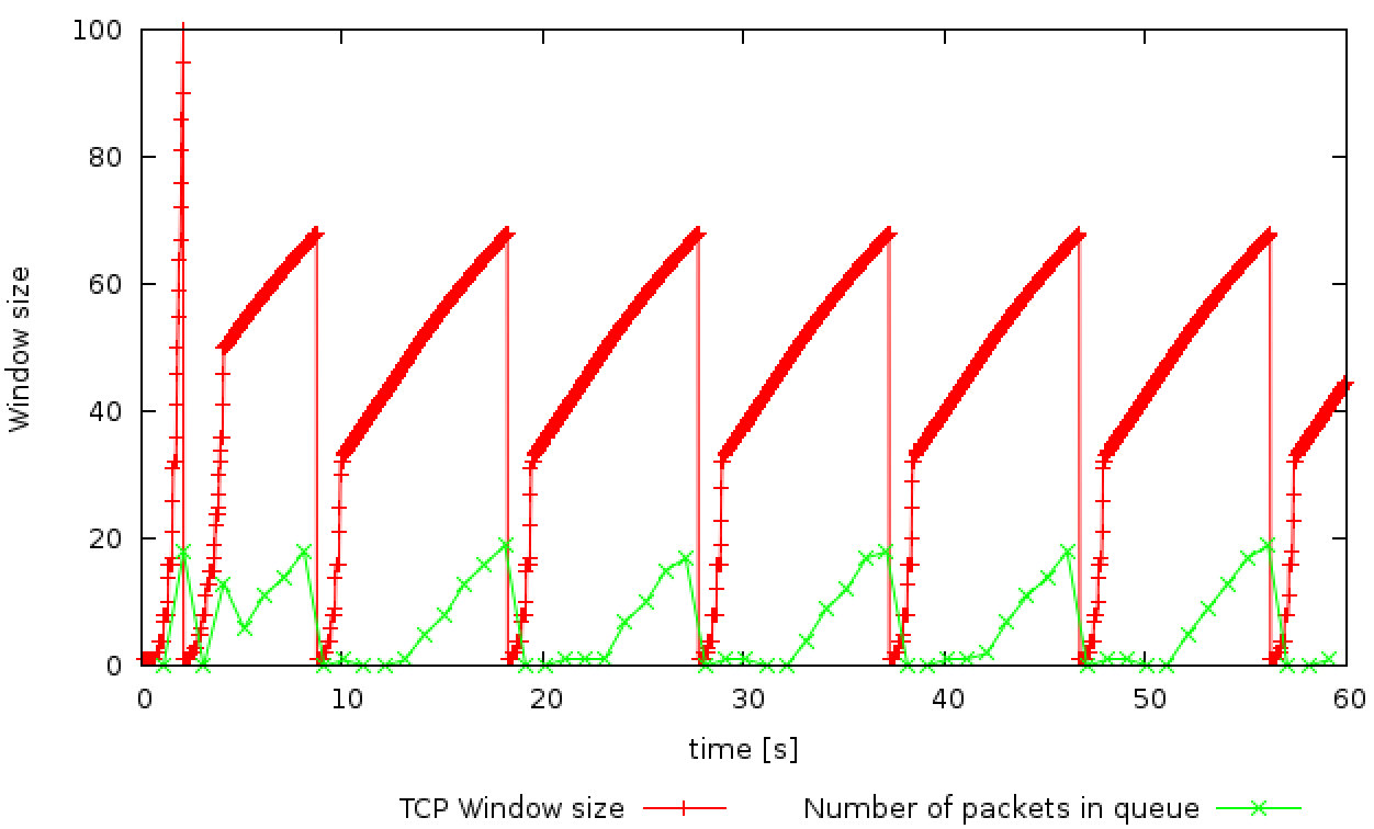
The congestion window grows up to 100 packets during the slow start phase, although the maximum congestion window we have set is 150 packets. This is because the maximum size of the queue is only 20 packets. Any additional packets are dropped. Thus, as the window size is ramping up the queue becomes full, packets get dropped which results in a congestion event (either timeout or triple duplicate acks - note that TCP Tahoe does not distinguish between the two) at the sender. The sender thus reduces the congestion window to 1 and the threshold to 1/2 the size of the window (i.e. 50 packets). The connection enters slow start and ramps up the window rapidly until it hits the threshold. Following this the connection transitions to congestion avoidance phase (i.e. AIMD). Eventually, the queue becomes full again, which creates packet loss. The connection transitions back to slow start and the sequence continues as observed in the graph.

Question 2. ( 1 mark )

The graph below shows the average and instantaneous throughput (in packets/sec) for the TCP connection.

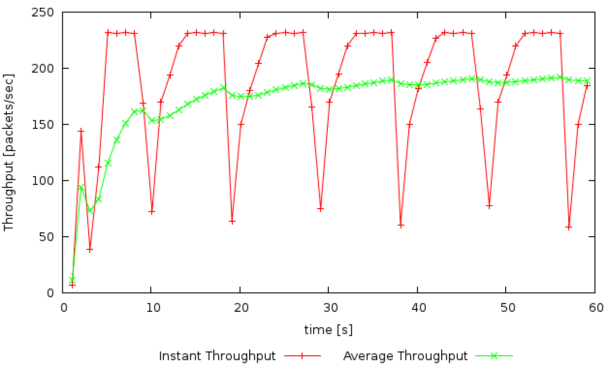
The average throughput of TCP in packets per second (pps) is 190 pps.

When it comes to calculating the throughput in bps, we have to make a distinction between:

1. The rate at which TCP transmits any kind of data; this includes header and payload data
2. The rate at which TCP transmits useful data; this only includes the payload.

Usually, it is the first definition that is more appropriate for throughput. Let's calculate the appropriate rates for both definitions of throughput, however:

1. According to the first definition, the throughput is 820.8 Kbps (190 x (500 + 40) x 8).
2. According to the second definition, the throughput is 760 Kbps (190 x 500 x 8).

Question 3. ( 2 marks )

As a general principle, when the maximum congestion window size becomes greater than the maximum queue size, some packets will get dropped and TCP will go back to slow start.

Here are a few interesting cases for the initial value of the initial maximum congestion window:

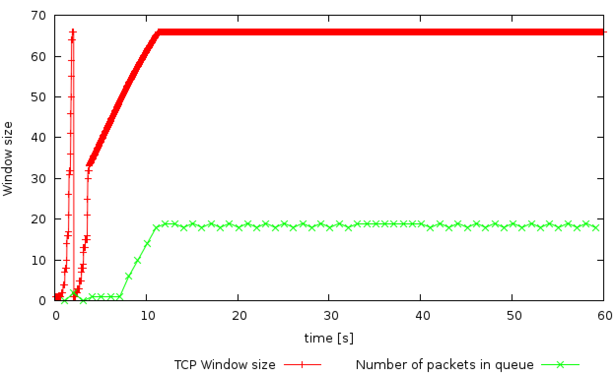
• Initial maximum congestion window <= 66: the oscillations stop after the first return to slow start. When we reduce the congestion window to half its size, this is enough to stabilise the number of packets in the sending queue; the queue never gets full, and so packets are not dropped anymore.
• Initial maximum congestion window <= 50 packets: TCP stabilises immediately.
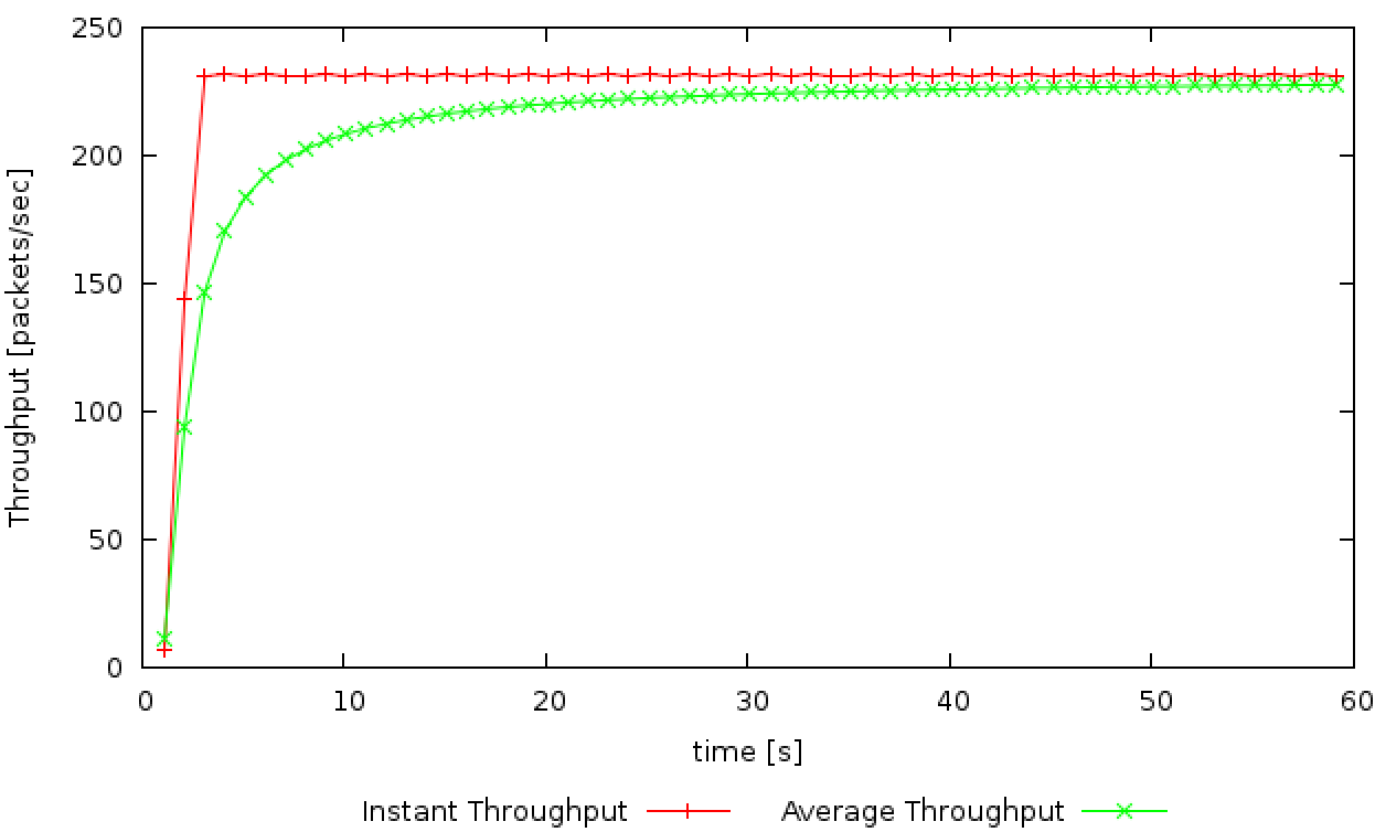
  At this point, the average packet throughput is close to 225 packets per second. The average throughput is 225x500x8=900 Kbps, which is almost equal to the link capacity (1 Mbps)

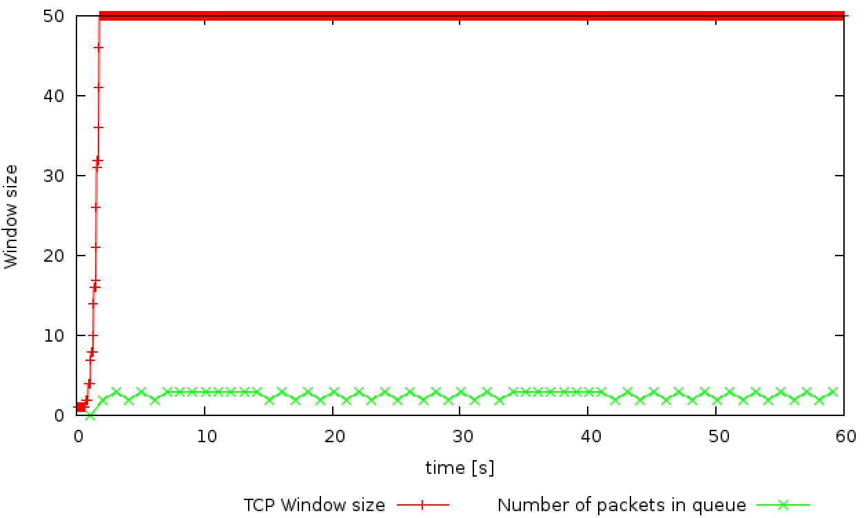
The graph below shows the window size when the initial max congestion window is set to 66

The graph below shows the window size when the initial max congestion window is set to 50.

The graph below shows the throughput when the initial max congestion window is set to 50.

TCP Tahoe vs TCP Reno

Question 4. ( 2 marks )

The following graph plots the congestion window and number of packets in the queue as a function of time.

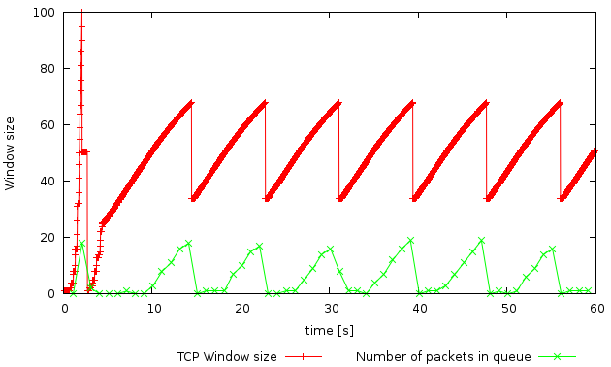
For the most part (except one timeout event at the start), the TCP connection does not enter slow start. Instead, the sender halves its current congestion window and increases it linearly, until losses starts taking place again. This pattern repeats. This implies that most of the losses are detected due to triple duplicate ACKs (as opposed to timeouts). This behaviour is different to TCP Tahoe where the window is reduced to 1 after each congestion event.

The graph below shows the average and instantaneous throughput (in packets/sec) for the TCP connection.

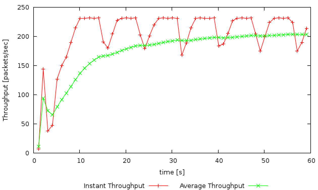
The throughput of TCP Reno is around 200 packets/second which is slightly higher than TCP Tahoe (which was 190 packets). This is because TCP Reno does not have to initiate slow start after each congestion event (unlike TCP Tahoe).

Exercise 2: Flow Fairness with TCP (2 marks)

The following graph plots the throughput for the 5 TCP connections.

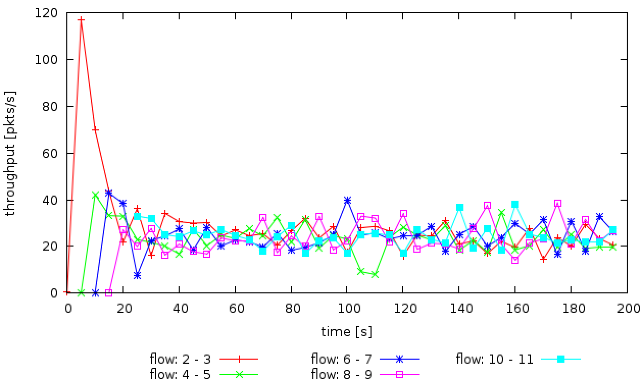
Question 1. ( 1 mark )

Once all five connections have commenced (i.e around 20 seconds), the throughput for all 5 connections is roughly similar (despite some fluctuations -which are a result of the ever changing congestion window as per AIMD). The approximate fair behaviour is a direct result of the AIMD congestion control algorithm employed by TCP. As was shown in the lecture, the AIMD strategy of adapting the window size achieves long-term fairness, when multiple flows share a bottleneck link. Since all flows experience the same network conditions, they will react in the same manner.

Question 2. ( 1 mark )

We can also observe from the above graph that when a new flow enters the network, the throughput of all pre-existing flows is reduced. This is because this new flow quickly ramps up its congestion window during slow start and creates congestion on the link. All existing TCP connections detect losses through duplicate ACKs and timeouts, and adapt the size of their congestion window in order to avoid overwhelming the network. This behaviour is fair, since once a new flow is added, the fair share of all existing flows should reduce accordingly.

Exercise 3: TCP competing with UDP (2 marks)

Question 1. ( 0.5 mark )

Recall that UDP does not employ any congestion control unlike TCP. This means that a UDP flow will not reduce its transmission rate in response to congestion. As such, we would expect that UDP would continue to transmit at its scheduled rate while TCP will try to settle in the leftover capacity.

The following graph plots the throughput for the two flows.

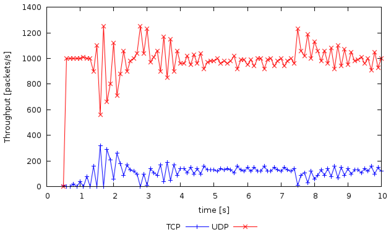
Question 2. ( 1 mark )

As expected, UDP achieves higher throughput than TCP, because it is not restrained by congestion control; it transmits packets at a constant rate, regardless of whether any of them get dropped. This is unfair to the TCP flow, which decreases its transmission rate when it detects congestion in the network (as detected by packet loss). Thus, the more aggressive UDP flows can starve TCP flows which traverse the same bottleneck links.

Question 3. ( 0.5 mark )

If UDP is used for transferring files, the advantage would be that the sender could keep transmitting unrestrained, irrespective of congestion. This may potentially (but not always) reduce the delay for transferring files. The disadvantage would be that the file transfer protocol running on top of UDP would need to implement reliable data transfer as UDP does not provide this service (unlike TCP).

If everyone started using UDP instead of TCP, then when faced with congestion, none of the flows would throttle their sending rate. Thus, there is a very strong possibility that parts of the Internet would encounter congestion collapse. Read this wikipedia article for a bit of historical background on what was taking place on the Internet in the 1980s, before congestion control was adopted.